AI Paint Defect Detection:
Seven Defects, One Edge Device
Seven Defects, One Edge Device: Lessons from Building an AI Paint Inspector
A project told through the decisions we made, the numbers that surprised us, and what we would do differently next time.
Most case studies list what was built. This one asks a more useful question: where did the real decisions sit? We trained a YOLO26s detector on seven paint defect classes and ran it on an NVIDIA Jetson Orin Nano. Here is the honest story of how, including the weak spots.
THE BRIEF
The project on one page
The goal was simple to state: take photos or live video of a painted surface and automatically mark visible paint defects. The model should detect seven categories (oil marks, orange peel, paint sagging, peel off, scratches, water marks and bubbling), be trained in the cloud, and run locally on a small edge computer that could sit near a production line.
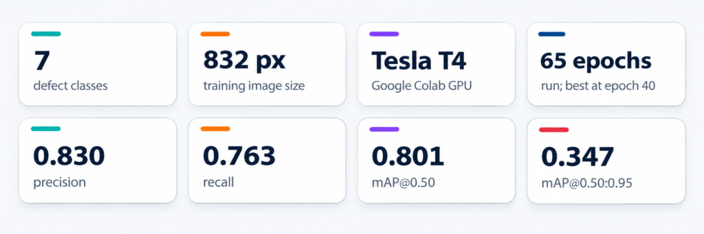
Figure 1. The project at a glance. Metrics are the recorded validation results of the training run.
Notice the shape of those numbers before we dig in. Precision and recall are respectable, and mAP@0.50 is a solid 0.80. But mAP@0.50:0.95 is only 0.35. That gap is the most interesting thing in the project, and we will come back to it.
THE ROUTE
From Colab to the factory floor
The pipeline has two halves connected by a single file. Training happens in Google Colab on a Tesla T4. When the best checkpoint is chosen, a file called best.pt is copied to the Jetson, where an inference script handles images, video files and a live camera.

Figure 2. The two halves of the system, connected by one model file.
DECISION 1
Define the problem as seven visible defects
The first choice was scope. Instead of a single “defect or no defect” classifier, the project uses object detection with seven classes. That tells an operator what is wrong and where, not just that something is.
Choice | Seven-class object detection on painted surfaces. |
Logic | Each defect type points to a different process problem, so labels carry more value than a yes/no flag. |
Cost | Defects are not equally “object-like”. Peel off has a clear shape; orange peel is a diffuse texture. One model must handle both. |
DECISION 2
Start from a public dataset
The training data came from a Roboflow paint defects dataset, downloaded as a ZIP and extracted to Google Drive with the standard train, valid and test layout and a data.yaml file defining the seven classes.

Figure 3. Image counts in the extracted dataset folders.
| Choice | Public Roboflow dataset, standard three-way split. |
| Logic | A ready-labelled dataset lets the team test the whole pipeline quickly, from training to edge deployment. |
| Cost | Public images may not look like your factory. Labelling consistency is also outside your control. |
Data hygiene note. The extracted folders contained 1,672 images, but the public Roboflow page showed 696. Before quoting a dataset size anywhere, verify the dataset version, file counts and possible duplicates.
DECISION 3
A small model, a larger image, a careful recipe
The model is YOLO26s, a compact variant suited to edge hardware. Training used an image size of 832 pixels, larger than the common default, because paint defects can be small and subtle. The recorded recipe is below.
Setting | Value | Setting | Value |
Model | YOLO26s (pretrained) | Optimizer | AdamW |
Image size | 832 px | Initial learning rate | 0.001 |
Batch size | 8 | Weight decay | 0.0005 |
Max epochs | 100 | Warm-up epochs | 3 |
Early-stop patience | 25 | Mosaic / MixUp | 0.5 / 0.0 |
Close mosaic | Last 10 epochs | Seed / AMP | 42 / enabled |
The early-stopping story. The run was set for up to 100 epochs but stopped at 65, because validation performance had not improved for 25 epochs. The best checkpoint came from epoch 40. This is early stopping doing its job: it keeps the best version and avoids over-fitting rather than signalling failure.
Choice | Small model, 832 px input, AdamW with light augmentation. |
Logic | Compact enough for an edge device, with enough resolution to see fine surface detail. |
Cost | Larger inputs slow inference. The 832 px setting is carried into deployment, so speed on the Jetson needs benchmarking. |
THE SCORECARD
What the numbers really say
Overall validation results were precision 0.830, recall 0.763, mAP@0.50 of 0.801 and mAP@0.50:0.95 of 0.347. Averages hide the story, though. Split them by class and two clear groups appear.
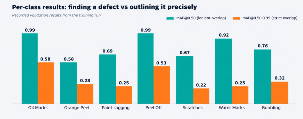
Figure 4. Per-class mAP at a lenient (0.50) and a strict (0.50:0.95) overlap threshold.
Two defects were easy
Oil Marks and Peel Off both reached about 0.99 mAP@0.50, with precision and recall near 0.97 or higher. They are visually distinctive: a dark, well-defined patch or a clearly lifted coating.
Three defects were hard
Orange Peel (0.578), Paint sagging (0.693) and Scratches (0.671) had the lowest mAP@0.50 and recall near 0.57 to 0.59. A scratch is thin, a sag can fade into the surface, and orange peel is a texture with no clear edge. Labelling such defects consistently is hard, which makes learning them harder.
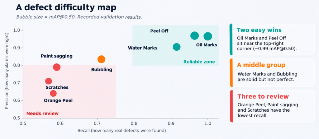
Figure 5. Precision and recall for each class. The bottom-left corner marks classes that need review.
Why is the strict score so much lower?
Water Marks is the clearest example. It scored 0.915 at the lenient threshold but only 0.248 at the strict range. The model finds water marks reliably, yet its boxes do not match the labelled outlines tightly, which is common when the defect has no sharp boundary. For an inspection system that only needs to flag an area, the lenient score matters most. For one that must measure defect size, the strict score matters more.
Takeaway. Look at which metric matches your use case. A system that raises an alert for human review and a system that measures defect area need different levels of box precision.
DECISION 4
Run it at the edge
After training, best.pt was downloaded from Colab and copied to the Jetson with scp (or a USB drive).
The inference script then handles three kinds of input:
- A live camera, with an annotated preview and a saved video (display mode required).
- A single image, with the annotated result saved to a results folder.
- A video file, processed and saved the same way.
Two parameters control behaviour: an image size of 832 (matching training) and a confidence threshold of 0.25, below which detections are discarded. The threshold is a dial between missed defects and false alarms and should be tuned on real images. Resource use can be watched with the tegrastats tool.
Choice | On-device inference on a Jetson Orin Nano. |
Logic | Local processing means low latency, no cloud dependency and images that stay on site. |
Cost | The software stack must match the installed JetPack. Do not blindly upgrade PyTorch or install a generic desktop CUDA build. |
FIELD NOTES
Troubleshooting the Jetson
Symptom | What to check first |
Model not found | The model path, and that best.pt exists in the expected folder. |
CUDA unavailable | JetPack release, PyTorch compatibility, and whether PyTorch reports CUDA as available. |
Install fails | The Jetson’s Python version. Use JetPack-compatible instructions or a pinned environment. |
Camera will not open | Device listing, permissions, other apps using the camera, and whether index 0 is the right one. |
No display over SSH | Use image or video mode without display, or a streaming approach. |
Low accuracy on new surfaces | Camera focus, lighting, resolution, labels, and review of false positives and negatives. |
Low frame rate | Watch tegrastats, try a smaller image size, then consider a compatible TensorRT export. |
REALITY CHECK
What these results do not tell us
- The figures are validation results on a public dataset, not a guarantee of performance on factory images.
- The test split should be reserved for final evaluation instead of repeated tuning.
- Inference speed on the Jetson has not been benchmarked here, so no frame-rate claim is made.
- Severity scoring, dashboards, sorting and process feedback are future extensions, not features of the current model.
- The dataset size discrepancy (1,672 versus 696) should be resolved before the dataset is cited.
NEXT STEPS
What we would do differently
Priority | Action | Why it matters |
1 | Review annotations for Orange Peel, Paint sagging and Scratches | These three classes show the lowest recall. |
2 | Collect images from the target line under controlled lighting | Closes the gap between public data and factory conditions. |
3 | Benchmark PyTorch on the Jetson, then test TensorRT | Establishes real frame rates before optimising. |
4 | Tune the confidence threshold on real images | Balances missed defects against false alarms. |
5 | Add severity estimation and a logging dashboard | Turns detection into quality intelligence. |
KEY TAKEAWAYS
Five lessons from the build
- Class difficulty is uneven. Distinct defects are easy; textures and thin marks are hard. Plan review effort accordingly.
- Pick the metric that matches the job. Alerting needs good detection; measuring needs tight boxes.
- Early stopping is a feature. The best epoch was 40 of a 65-epoch run.
- The edge is an engineering problem, too. Software compatibility on the Jetson takes as much care as training.
- Be honest about limits. Public-data validation is a starting point, not a factory certificate.